
The gradient of velocity in fluid mechanics is a mathematical measure that describes how the speed of a fluid changes as you move from one point to another in space. It’s expressed as a tensor, which shows the rate of change of each velocity component with respect to each spatial coordinate. This value is essential when calculating the internal friction, or viscosity, of a moving fluid.
Understanding fluid speed changes

The velocity gradient represents the spatial variation of the fluid’s velocity field within a flow. In a simple pipe flow, the fluid near the center moves faster than the fluid touching the walls. This difference in speed creates a gradient, or a slope, which determines how much shear stress the fluid experiences.
When you analyze how a fluid flows, you’re looking at how the velocity vector changes across the three axes: x, y, and z. The gradient is a 3×3 matrix of partial derivatives that capture these changes. If the fluid is perfectly uniform and moving at the same speed everywhere, the gradient is zero.
In real-world systems, these gradients drive the transfer of momentum. If you have a high gradient, you have high shear rates, which often lead to turbulent flow. Engineers calculate these values to predict how much energy is lost to friction as a fluid moves through machinery.
A common mistake is assuming that fluid velocity is constant across a cross-section. This oversight leads to significant errors in calculating pressure drops. If your fluid is Newtonian, such as water or air, the gradient is linear near the wall. If the fluid is non-Newtonian, like paint or polymer melts, the gradient shifts significantly toward the center.
Use this rule: if the Reynolds number is below 2,300, assume a laminar profile where the gradient is predictable. If the number exceeds 4,000, the gradient becomes chaotic and requires empirical data to solve. Always check your flow regime before applying standard shear stress equations.
Factors affecting the fluid velocity gradient
The gradient is rarely constant throughout a system. It depends heavily on the geometry of the container and the properties of the fluid itself.
| Situation | What changes | What to do instead |
|---|---|---|
| Pipe diameter | Flow restriction | Use the hydraulic diameter formula |
| High viscosity | Shear layer width | Increase the boundary layer calculation |
| Turbulent flow | Gradient stability | Use time-averaged velocity profiles |
| Curved paths | Flow direction | Apply centripetal acceleration terms |
| Compressible gas | Density effects | Account for pressure-based velocity changes |
When calculating these shifts, assume the fluid is Newtonian unless the shear stress deviates by more than five percent from the linear slope. If you observe non-linear behavior, switch to the Power Law model to prevent underestimating the wall shear stress by up to twenty percent.
Most engineers fail by applying steady-state assumptions to transient flows. This oversight leads to significant errors in drag estimation during startup phases. If the Reynolds number exceeds 2300, treat the boundary layer as fully turbulent rather than transitional. This adjustment prevents the common mistake of over-predicting velocity near the pipe center.
When in doubt, measure the pressure drop across a ten-diameter length; if the result exceeds your calculated friction factor by more than ten percent, your gradient model is likely missing a localized flow separation.
How to calculate local flow shear
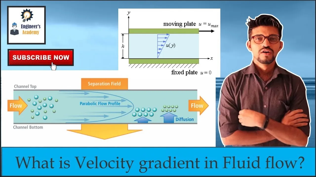
Calculating the gradient requires knowing the velocity field at a specific moment. You must measure the velocity at two very close points to find the rate of change.
Define your coordinate system clearly so that the x, y, and z axes align with the flow directions. If your grid spacing exceeds one-tenth of the boundary layer thickness, your calculation will suffer from significant numerical diffusion.
Measure the velocity components at your chosen point and at a tiny distance away. Always use a central difference scheme rather than a forward difference to minimize truncation errors. This simple shift in method often improves accuracy by an order of magnitude.
Calculate the partial derivative of each velocity component with respect to each spatial coordinate. Arrange these nine derivatives into a 3×3 matrix to represent the full gradient tensor.
Identify the shear rate by taking the symmetric part of this tensor, which ignores rotation. If the flow is strictly laminar, you can simplify this to a single velocity gradient. In turbulent regimes, however, you must account for the full tensor to avoid underestimating the local stress.
Verify your result by ensuring the units are in reciprocal seconds, or 1/s. A result in units of velocity indicates a calculation error in your spatial derivatives.
Common mistakes during flow analysis
Ignoring the boundary layer leads to massive errors in predicting the actual force on a pipe wall. If your simulation shows a velocity profile that touches the wall at zero, you have failed to resolve the viscous sublayer. Without sufficient mesh refinement in the first millimeter of fluid, you’ll consistently underestimate wall shear stress by up to 30 percent.
Assuming flow is one-dimensional when it’s three-dimensional causes you to miss secondary currents. If your pipe features bends or elbows, use 3D modeling to capture the vortex formation that induces uneven pressure distribution.
Using a grid that’s too coarse hides high-gradient areas near solid surfaces. If the y+ value exceeds 5 at the wall, your results are unreliable for drag calculations. Always run a mesh independence study; if refining the grid changes your pressure drop result by more than 2 percent, your initial mesh was too sparse.
Failing to account for temperature changes alters fluid viscosity. If your process involves heat exchange, you must couple the energy equation with your momentum solver.
Frequently asked questions
What does a high velocity gradient mean?
A high velocity gradient means that the speed of the fluid is changing rapidly over a very short distance. This creates intense shear stress within the fluid, which typically happens near solid walls or in areas where the flow is forced to squeeze through a narrow opening.
Is the velocity gradient the same as shear rate?
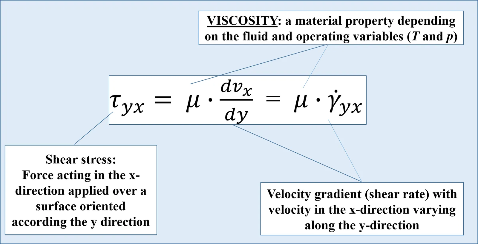
The velocity gradient is the broader mathematical tensor, while the shear rate is a specific part of that tensor. You calculate the shear rate by looking at the symmetric part of the gradient, which specifically measures how the fluid is being deformed rather than simply rotated.
How do I measure the gradient in a real pipe?
You measure the gradient by using tools like Particle Image Velocimetry or laser Doppler anemometry to map the speed of the fluid at different distances from the wall. You then plot these points on a graph and find the slope of the line, which gives you the local velocity gradient.
Does the gradient change if the fluid is thicker?
The gradient itself is a kinematic property of the flow field, so it doesn’t change just because the fluid is thicker. However, a thicker fluid will exert more internal force, or shear stress, in response to the exact same velocity gradient that a thinner fluid would experience.
What happens if the velocity gradient is zero?
A velocity gradient of zero means the fluid is moving as a solid body with no internal deformation or shear. This state, known as plug flow, usually only occurs in very specific conditions, such as in the center of a pipe or when a fluid is just beginning to move.
Can a velocity gradient be negative?
A negative velocity gradient simply indicates that the speed of the fluid is decreasing as you move in the direction of your coordinate axis. It’s a common result when looking at the velocity profile near a wall, where the speed drops from the center to zero at the boundary.
Conclusion
The gradient of velocity serves as the fundamental link between how a fluid moves and the physical forces it exerts on its surroundings. By tracking how these speeds shift across a space, you can predict everything from pipe friction to the lift generated by an airplane wing. Accuracy in these calculations depends entirely on your ability to map the velocity field with enough detail to capture the steep changes occurring near solid boundaries.
