
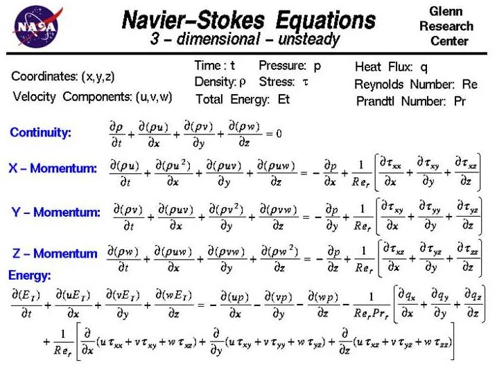
The navier stokes equations are a set of partial differential equations that describe how the velocity, pressure, temperature, and density of a moving fluid are related. These equations express Newton’s second law of motion for fluids, accounting for forces like viscosity, pressure, and external gravity. They serve as the foundation for modern fluid mechanics, allowing engineers and scientists to predict how liquids and gases flow through pipes, around airfoils, or across weather systems.
These equations work by balancing the forces acting on a tiny volume of fluid. If the fluid is incompressible, like water, you use a simplified version that assumes density stays constant. If the fluid is compressible, like air moving at high speeds, you must include density changes in your calculations.
The most common mistake people make is trying to solve these equations analytically for every situation. In reality, exact solutions only exist for very simple, symmetric flows. For complex real-world problems, such as air flowing over a car, you must use numerical methods and powerful computers to find an approximate result.
How Navier Stokes equations model fluid motion

To use these equations effectively, you must define the boundaries of your system and the properties of the fluid involved. Because these equations are highly complex, most practical work involves computational fluid dynamics, which breaks the space into a grid of small cells to estimate the flow.
- Define your fluid properties, specifically the density and dynamic viscosity, which change based on the material and temperature.
- Set the boundary conditions for your simulation, such as the velocity of the fluid at the walls and the pressure at the inlet.
- Choose a numerical solver, such as a finite volume method, to approximate the derivatives within the equations.
- Run the simulation through an iterative process until the changes between steps fall below your chosen tolerance level.
- Validate your results against experimental data, as numerical errors can accumulate in complex turbulence models.
Tip: Always ensure your grid is fine enough to capture small-scale features. If the mesh is too coarse, you’ll lose accuracy in areas where the flow changes quickly.
Tip: If you’re working with high-speed gases, you must include the energy equation to account for heat transfer. This adds another layer of complexity that requires specialized software to manage.
Time required for fluid analysis
The time it takes to solve these equations depends on the complexity of the geometry and the required level of detail. Simple steady-state problems might take minutes, while highly turbulent, time-dependent simulations can run for weeks on supercomputers. According to the NASA Glenn Research Center, these equations are the primary tools used in aerospace engineering to understand aerodynamic performance.
| Situation | Typical Time | What changes it | What to watch for |
|---|---|---|---|
| Simple pipe flow | Minutes | Pipe length | Pressure drop |
| Steady-state airfoil | Hours | Grid density | Stall points |
| Turbulent combustion | Days/Weeks | Reaction models | Heat release |
If your simulation is taking significantly longer than expected, check for “stiff” equations where the time step is forced to be extremely small to maintain stability. You may need to adjust your numerical scheme or simplify the physical model.
A common mistake is failing to refine the mesh only where gradients are highest. If you apply a uniform mesh to the entire domain, you waste cycles on stagnant flow regions. Instead, use adaptive mesh refinement to concentrate cells near boundary layers.
If your simulation runs for more than 48 hours without reaching convergence, check your residuals. If residuals oscillate rather than drop, your time step is likely too large for the physics. Cut your time step by half; if the residuals stabilize, you have found the threshold. If they remain erratic, your boundary conditions are likely physically inconsistent.
Signs of a completed simulation
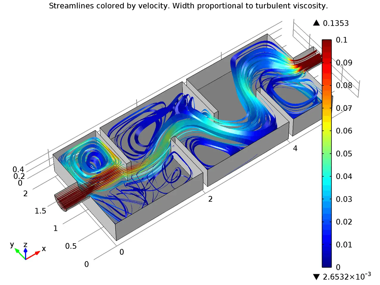
A simulation is considered done when the solution reaches a steady state or when the time-averaged results show consistent patterns. You can look for “residuals,” which are values that measure how much the equations are failing to balance at each point. When these residuals drop below a set threshold, such as 10^-6, the solution is typically considered converged.
Monitor specific physical values, like the drag force on an object. If this value stops changing by more than 0.1% over 500 iterations, your simulation has likely reached a stable result.
Commonly, engineers mistake high residual drops for accuracy, even when local flow features remain unstable. If your residuals oscillate within a tight band rather than dropping, don’t force convergence by tightening tolerances. This indicates the flow is naturally unsteady. In this case, switch to a time-accurate solver.
You must then average your data over at least three full cycles of the observed oscillation to obtain a valid result. If you ignore these fluctuations, you risk capturing a false steady state that misrepresents the actual physical load.
Errors that ruin flow models
Ignoring turbulence effects leads to catastrophic failures in predictive accuracy. If you treat a turbulent flow as a simple laminar one, your drag and heat transfer estimates will be completely wrong. Always use a turbulence model appropriate for the Reynolds number of your specific application. If your Reynolds number exceeds 4,000, abandon laminar assumptions entirely or risk underestimating skin friction by as much as 30 percent.
Poor mesh quality remains the primary cause of solver divergence. Using cells with skewness values above 0.85 introduces artificial numerical diffusion that masks the true physics. Ensure your grid is orthogonal and refined in areas where the velocity changes rapidly, such as near solid walls. If your y+ value isn’t calibrated to the boundary layer thickness, your wall functions will produce garbage data.
Incorrect boundary conditions force the math to yield an impossible result. Always verify that your inputs represent the physical reality of your system.
Related guides
- 10 Best Phosphate Removers to Keep Your Pool Clear in 2026
- Best Drain Unblockers: How to Clear Clogs Effectively in 2026
- 8 Perfect Weekly Pool Chemical Reviews for Clear Water in 2026
Frequently asked questions
Can the navier stokes equations be solved exactly?
No, they can’t be solved exactly for most real-world applications because they’re non-linear and highly complex. Mathematicians have found exact solutions only for highly simplified cases with perfect symmetry or very low speeds. For almost every practical use, engineers rely on numerical approximations and high-performance computing to find results that are close enough to reality to be useful for design and safety analysis.
Is it safe to use these equations for structural design?
Yes, it’s safe, but you must use them as part of a larger analysis that includes structural mechanics. These equations provide the fluid forces, such as wind pressure, which you then apply as loads on a structure. You should always consult professional structural engineering standards to ensure your load assumptions align with safety codes for your specific region and type of building.
How long does a typical fluid simulation take?
It takes anywhere from a few minutes to several weeks depending on the number of cells in your grid and the time-stepping method used. A simple 2D steady-state problem might finish in under an hour on a standard desktop. However, a full 3D simulation of a complex engine or aircraft requires massive parallel processing on a cluster to reach a result in a reasonable timeframe.
What happens if the fluid is compressible?
If the fluid is compressible, the density is no longer constant, and you must add the continuity and energy equations to your calculation. This happens when gas speeds reach a significant fraction of the speed of sound, causing pressure waves. You’ll need to account for these changes in density and temperature, which makes the system of equations much more difficult to solve than those for incompressible liquids.
Why are these equations so hard to solve?
They’re hard to solve because they’re non-linear, meaning the output isn’t directly proportional to the input. This non-linearity creates turbulence, where tiny changes in the starting conditions lead to vastly different outcomes over time. This sensitivity makes it difficult for computers to track every single swirl and eddy in a fluid, requiring advanced algorithms to provide stable and accurate predictions.
Conclusion
While these formulas look intimidating, they’re essential for solving real-world challenges. You don’t need to be a math genius to appreciate how they shape our world, from designing fuel-efficient planes to predicting storms. If you’re curious to learn more, try exploring some basic fluid simulations online; you’ll see them in action.
