
Neumann boundary conditions are mathematical constraints that specify the derivative of a solution at the boundary of a domain. Instead of fixing the value of the function itself, these conditions dictate the rate of change or the flux across the edge. Engineers and scientists use them to model physical systems where the flow, heat, or force at the surface is known rather than the absolute state.
These conditions are essential when you’re modeling systems like heat transfer or fluid flow where the gradient matters more than the specific value. If you know the heat flux entering a wall, you apply a neumann condition to define that flow rate. The most common mistake is confusing these with dirichlet conditions, which fix the actual value at the boundary. Mixing these up leads to incorrect physical models and results that don’t match reality.
Applying Neumann boundary conditions
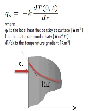
When you apply these conditions, you’re telling the computer how much stuff moves through a border. If the gradient is zero, the boundary is insulated or closed. Nothing enters or leaves.
A common mistake is mixing up total power with flux density. Applying 500 watts to a face instead of dividing by its area overloads that surface. The solver then produces temperatures that melt your geometry in seconds.
- Identify the boundary where you have information about the flux or rate of change.
- Define the derivative value at that specific surface, such as heat flux in watts per square meter.
- Apply the constraint to your numerical solver, ensuring units match your coordinate system.
- Check if your model requires a reference value. These conditions only define the shape of the solution, not its absolute level.
If you assign inward flux on every single face of a sealed domain, energy accumulates forever. The temperature climbs without limit. At least one boundary must let energy out, or you must fix a starting temperature somewhere.
Tip: If you’re working with partial differential equations, always verify that your boundary conditions are consistent with the governing physics of your problem.
Tip: If your solver fails to converge, ensure that your boundary flux values are physically possible for the material properties you have defined.
Understanding time and complexity
The time required to compute a solution depends on the grid size and the type of solver you choose. Simple problems with linear equations solve in seconds, while complex fluid simulations take hours or days on high-end hardware.
| Situation | How long | What changes it | What to watch for |
|---|---|---|---|
| Simple 2D heat flow | Seconds | Grid density | Stability of the gradient |
| Complex 3D fluid flow | Hours | Mesh refinement | Turbulence at the edges |
| Steady-state analysis | Minutes | Iterative solver | Convergence rate |
| Transient simulation | Days | Time-step size | Cumulative error drift |
If the simulation runs for much longer than expected, check for a non-physical gradient value that prevents the solver from reaching a steady state.
Most users mistakenly refine the entire mesh when only a specific boundary needs higher resolution. This mistake often triples your compute time without improving the result. If your simulation stalls, isolate the high-gradient region and apply local refinement instead of global changes.
Use this rule to gauge your timeline: if your time-step is smaller than the smallest cell size divided by the fluid velocity, your model will likely crash or diverge. If you see the error residual oscillating rather than dropping, your solver is fighting an unstable mesh geometry. In these cases, switch from a second-order scheme to a first-order upwind method to force convergence, even if you sacrifice some spatial accuracy.
Identifying when the solution holds
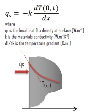
You know the simulation is correct when the flux at the boundary matches your input parameters. If you set a heat flux of zero, the temperature gradient at that edge must be perfectly flat. A key sign of a finished, stable solution is that the residuals—the difference between successive iterations—drop below your set tolerance limit.
Watch the convergence plot for oscillations. If the residuals plateau rather than dropping, the simulation has stalled. This usually signals that your mesh is too coarse to capture the physics at the boundary.
When signs disagree, such as the boundary flux not matching your input, perform a grid independence test. Refine your mesh to see if the boundary derivative stabilizes. If it does not, the issue likely sits in your formulation of the boundary condition itself.
Always consult the technical manual of your specific software to see how it handles derivative definitions. Some tools require a sign convention that differs from standard calculus notation. If you see a negative flux where you expect a positive value, invert the sign in your input file before re-running the solver.
Common errors in boundary setup
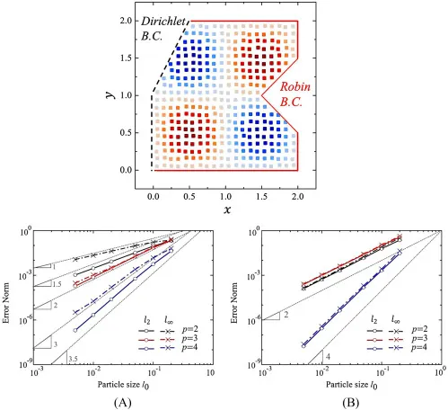
People often flip the direction of the flux, causing energy to enter the system when it should be leaving. Always check your coordinate system and ensure the outward normal vector aligns with your intended flow direction. If your simulation shows a temperature spike at the boundary, you have likely reversed the sign.
Using mismatched units between the domain and the boundary condition leads to wild, non-physical results. Verify that your flux units, such as heat per unit area, are mathematically compatible with the units used for the spatial dimensions. A common mistake is mixing imperial and metric inputs, which often results in errors scaling by orders of magnitude.
Because these conditions only define the derivative, the absolute value of your solution can drift. You must provide at least one point of reference or a Dirichlet condition elsewhere in the domain to anchor the solution to a real-world value. If your model fails to converge, add a single fixed-value constraint at the center. This anchors the floating variable and prevents the solver from oscillating indefinitely.
Related guides
- What Is the Moment of Inertia Matrix: A Clear Guide
- 10 Best Phosphate Removers to Keep Your Pool Clear in 2026
- How Current Foldback Protects Power Supplies: A Clear Guide
Frequently asked questions
Can neumann boundary conditions be time-dependent?
Yes, these conditions can change over time if your physical system has a flux that varies. If you’re modeling a heating element that turns on and off, you must define the derivative as a function of time. The solver will then update the flux at each time step, which requires a transient analysis setup rather than a steady-state one.
Is it safe to use zero flux?
Yes, a zero-flux condition—often called a homogeneous condition—is safe and common for insulated boundaries. It simply means the derivative is zero, effectively sealing the boundary against any flow or transfer. You should use this whenever you know a surface is perfectly isolated from the surrounding environment, as it prevents any energy or mass from crossing that specific line or plane.
How do I choose between dirichlet and neumann?
Use dirichlet conditions when you know the exact value, such as a fixed temperature, and neumann conditions when you know the rate of change or flux.
What happens if I use both on the same point?
Using both conditions at the exact same point creates a conflict that usually makes the system impossible to solve. This is known as an over-determined system, and numerical solvers will often throw an error or produce nonsense. You must choose one condition per boundary section to maintain the mathematical integrity of your model and ensure the solver has a clear path to a valid solution.
How long does a mesh convergence test take?
A mesh convergence test usually takes two to three times longer than your initial simulation run. You must run the simulation at a coarse, medium, and fine mesh setting to see if the boundary results stop changing. Once the output value stays the same regardless of how much you refine the mesh, you know your results are stable and accurate.
Conclusion
The accuracy of your simulation depends heavily on how well you define these constraints at the start. If you input the wrong derivative, the entire model will provide a result that looks correct but lacks any physical meaning. Always double-check your flux directions and units before you begin a long simulation run to save yourself from wasted time and effort.
